Difference between revisions of "Simulation Tutorial"
(→Select Analog Environment) |
m (→Adding Model Library Files) |
||
| (136 intermediate revisions by 7 users not shown) | |||
| Line 1: | Line 1: | ||
| − | + | There are many ways to simulate from Virtuoso. Which one is best depends on your PDK and your final goals. | |
| − | + | ||
| − | + | ||
| − | + | ||
| − | + | == Setting up analogLib == | |
| + | Before you start virtuoso, make sure to add the analogLib to your libraries. Do this by editing cds.lib in your home directory (or in the project directory). You should see something like this: | ||
| + | DEFINE analogLib $CDSHOME/tools/dfII/etc/cdslib/artist/analogLib | ||
| + | DEFINE US_8ths $CDSHOME/tools/dfII/etc/cdslib/sheets/US_8ths | ||
| + | DEFINE basic $CDSHOME/tools/dfII/etc/cdslib/basic | ||
| + | DEFINE cdsDefTechLib $CDSHOME/tools/dfII/etc/cdsDefTechLib | ||
| + | DEFINE NCSU_TechLib_FreePDK45 $PDK_DIR/ncsu_basekit/lib/NCSU_TechLib_FreePDK45 | ||
| + | DEFINE NCSU_Devices_FreePDK45 $PDK_DIR/ncsu_basekit/lib/NCSU_Devices_FreePDK45 | ||
| + | DEFINE cmpe_222_lib /mada/users/rsankara/cmpe_222_lib | ||
| − | |||
| − | + | In case your cds.lib does NOT have analogLib or one of the above libraries, then add it as follows: | |
| + | DEFINE analogLib $CDSHOME/tools/dfII/etc/cdslib/artist/analogLib | ||
| − | + | Save the file and start virtuoso. You should see a new library in the library manager. | |
| − | + | ||
| − | + | ||
| − | + | ||
| − | + | == Select Analog Environment == | |
| + | With the schematic file open, hspice can be invoked from within Virtuoso. | ||
| + | :Select <b>Launch → ADE L</b>. <br> | ||
| + | == Select Simulator (<nowiki>hspiceD</nowiki>) == | ||
| + | Virtuoso Analog Design Environment supports various simulators such as hspiceD, Spectre, and Ultrasim. hspiceD was previously chosen. Now, run | ||
| + | :Select<b> <nowiki> Setup → Simulator/Directory/Host. </nowiki> </b> | ||
| + | A follow up window will pop up giving your simulator options. Select '''hspiceD'''. Also specify a run directory. Press ok. | ||
| − | |||
| − | |||
| − | <b> | + | <b>Simulation Run Directory</b> indicates where your simulation files will be stored. |
| − | The generated netlist file will be stored within | + | The generated netlist file will be stored within in a file called "netlist". |
| + | All of the other options necessary for running the simulation are stored in this directory as well in the form of separate files like netlistHeader, netlistFooter. | ||
| + | When you run the simulation, all the options are put together by the simulator. | ||
| + | This is useful for storing separate simulation setups for different parts of your design. | ||
| − | |||
| − | |||
| − | == Choosing Analysis Length == | + | == Choosing Analysis Type and Length == |
From the Analog Environment window | From the Analog Environment window | ||
:Select <b>Analysis → Choose </b> | :Select <b>Analysis → Choose </b> | ||
| − | + | Make sure to select tran and specify an appropriate stop time and time step (example 1ns). | |
| − | + | The start time is typically 0. | |
| − | + | Be sure to choose a stop time that is greater than the period of the input signal. | |
| + | Hspice supports the SI prefixes so 500n would be 500 nano seconds. | ||
| − | |||
| − | |||
| − | |||
| − | |||
== Adding Model Library Files == | == Adding Model Library Files == | ||
The next step is to add the spice data for the simulator. | The next step is to add the spice data for the simulator. | ||
| − | :Select <b> Setup → Model | + | :Select <b> Setup → Model Library Setup </b>. |
| − | We will be adding the data for the | + | We will be adding the data for the NMOS and PMOS transistor. |
| − | |||
| + | If you are using FreePDK as your Process Design Kit, | ||
| + | Click on <i>Add File</i> and add these files: | ||
| − | + | $PDK_DIR/ncsu_basekit/models/hspice/tran_models/models_nom/NMOS_VTL.inc | |
| − | + | $PDK_DIR/ncsu_basekit/models/hspice/tran_models/models_nom/PMOS_VTL.inc | |
| − | |||
| − | |||
| − | |||
| − | + | Select <b> OK </b> when finished. | |
| − | + | These paths will be automatically written as ".include" into a file called input.ckt | |
| − | + | ||
| − | + | ||
| − | + | ||
| − | |||
| − | + | If you are using SCMOS(TSMC_02d) as your Process Design Kit, | |
| − | + | ||
| − | + | ||
| + | Click on <i>Add File</i> and add these files instead: | ||
| + | |||
| + | /mada/software/techfiles/ncsu/models/hspice/public/tsmc18dP.m | ||
| + | /mada/software/techfiles/ncsu/models/hspice/public/tsmc18dN.m | ||
| + | |||
| + | |||
| + | Select <b> OK </b> when finished. | ||
| + | |||
| + | |||
| + | |||
| + | Perform this '''Adding Model Library Files''' step only for the process you are supposed to use. Adding multiple process files may lead to simulation problems. | ||
| + | |||
| + | == Running Simulation == | ||
| + | |||
| + | To run a simulation, first select the type of analysis in <b>Analysis → Choose...</b> For a transient, specify the stop time (e.g. 1n). | ||
| + | |||
| + | It is easier to not add voltage sources to the inputs directly and instead make stimulus in a file. You can edit a stimulus file directly and include it in your simulation. | ||
| + | Create a text file named ''stimulus.sp'' in your simulation directory and create something like this in it: | ||
| + | |||
| + | // Stimulus Statements Hspice format | ||
| + | .global VDD! vdd! GND! gnd! | ||
| + | vdd vdd! 0 vhigh | ||
| + | .param vhigh=1200mV | ||
| + | .param vlow=0 | ||
| + | .param tdelay=0n | ||
| + | .param trise=5p * pick a reasonable value | ||
| + | .param tfall=5p * pick a reasonable value | ||
| + | .param tpulse = 10n | ||
| + | v_A A 0 pat (vhigh vlow tdelay trise tfall tpulse b01010101 rb=1 r=1) | ||
| + | C_Z Z 0 100fF * pick a reasonable value | ||
| + | |||
| + | The above statements define the global signals, define the '''vdd''' voltage using a parametrized statement and also some timing values. | ||
| + | These statements may also be written in the netlist file itself if you wish to have it all in a single file. | ||
| + | The '''.param''' statements above are used for parameterizing simulation variables. This way, if you wish to change some values for simulation, you only need to change it in the '''.param''' statement and it will take effect throughout. | ||
| + | The '''v_A''' is a voltage source statement producing a bit stream of 01010101 as stimulus with rise,fall and pulse width times defined in the '''.param''' statements. | ||
| + | Save the file you have now created as stimulus.sp and store it in your simulation directory. | ||
| + | |||
| + | To specify the stimulus, select <b>Setup → Simulation Files..</b>. and provide the path to your ''stimulus.sp''. | ||
| + | |||
| + | |||
| + | For more information on Hspice commands you can look at the manual: | ||
| + | |||
| + | /projects/cmpe122/software/I-2013.12-1/hspice/docs_help/hspice_sa.pdf | ||
| + | |||
| + | == Ouput Window == | ||
| + | Before Running, select <b>Output → Save All...</b> to save all schematic data. (Note, this might not be best on big designs!) Or, you can select <b>Outputs → To Plot → Select on Schematic</b> and then click on all of the items on the schematic. | ||
| + | |||
| + | Then, | ||
| + | :Select <b> Simulation → Run</b> | ||
| + | This will generate the netlist file, run the simulation, and save the results for the waveform viewer. You should re-run this every time you change your schematic. | ||
| + | |||
| + | You can also select <b>Simulation → Create Raw</b> to create the raw simulation file for debugging. You should be able to see your include stimulus, netlist, and a bunch of other stuff. | ||
| + | |||
| + | If this pops up a window that says it failed, fix the previous options. You need to debug this by looking at the output of the simulator in si.log (which is the output of running the simulator, if the simulator failed to run) or si.out (which is the actual simulator output if it ran successfully, but simulation may have failed). This will show you if it even got to the point of running the simulator. | ||
| + | |||
| + | |||
| + | If it succeeded, you can select <b> Tools → Waveform </b>. When you do this, you get three windows: | ||
| + | |||
| + | [[Image:waveform_graph.jpg|400px]] | ||
| + | [[Image:waveform_browser.jpg|400px]] | ||
| + | [[Image:waveform_results.jpg|400px]] | ||
| + | |||
| + | Select the "File Open" icon and then find the appropriate "raw" result file in the browser. This should open the data in the browser. Double click on the transient simulation directory and you should see signal names that correspond to your design. Double click on "A" to add it. Change the upper right option to "Append" and double click on "Z" to add it as well. If you don't change the option, it will replace the A waveform with Z. If there are problems with vdd! and gnd! you can debug that here. | ||
| + | |||
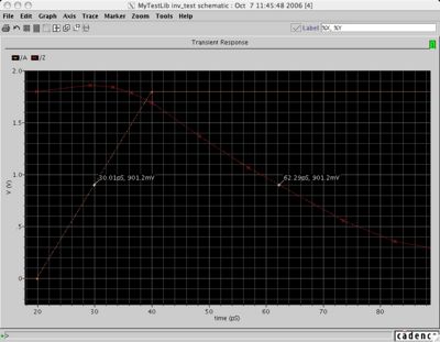
| + | You should get something that looks similar to this in the graph window: | ||
[[Image:output_waveform.jpg|400px]] | [[Image:output_waveform.jpg|400px]] | ||
| + | |||
| + | Note that your signals should always rise to full vdd (1.2V) and down to gnd (0V) or else something is wrong with your logic. This is CMOS so everything is "rail to rail". It is likely an unconnected supply voltage or floating body. | ||
== Waveform - Zooming and Trace == | == Waveform - Zooming and Trace == | ||
| Line 80: | Line 143: | ||
=== Zoom === | === Zoom === | ||
| − | :Select <b> Zoom → X Zoom </b> | + | :Select <b> Zoom → X Zoom </b>. |
:Now click and drag in the waveform window to select the x-range you want to zoom to. | :Now click and drag in the waveform window to select the x-range you want to zoom to. | ||
| Line 88: | Line 151: | ||
[[Image:zoom_waveform.jpg|400px]] | [[Image:zoom_waveform.jpg|400px]] | ||
| − | :Click on one of the waveforms in the window. This places a small label on the waveform. You can drag this marker anywhere on the waveform | + | :Click on one of the waveforms in the window. This places a small label on the waveform. You can drag this marker anywhere on the waveform. |
| + | |||
| + | === Separate Windows === | ||
| + | :Sometimes the window will get too cluttered. You can plot each signal in a separate window by clicking the 4th icon in the toolbar from the left to put it in "Strip Mode". | ||
| + | |||
| + | === Reloading === | ||
| + | :If you make a change and resimulation, you can simply click <b> File → Reload </b> | ||
| + | |||
| + | === Exporting Tip === | ||
| + | :If you intend to export the plot, it would be wise to change the background color to something other than black. In addition you can change the width of the lines by right clicking on the line and selecting properties. | ||
| + | |||
| + | == Power/Energy Analysis == | ||
| + | |||
| + | To enable power analysis in hspice, add this statement to your stimulus file: | ||
| + | |||
| + | .measure tran toplvl_avg_power avg power from=0ns to=100ns | ||
| + | .measure tran toplvl_avg_energ integ power from=0ns to=100ns | ||
| + | .measure tran toplvl_avg_current avg I(VDD) from=0ns to=100ns | ||
| + | |||
| + | For more information on the .measure syntax, please refer hspice user guide at: | ||
| + | /projects/cmpe122/software/synopsys/I-2013.12-1/hspice/docs_help/hspice_sa.pdf | ||
| + | |||
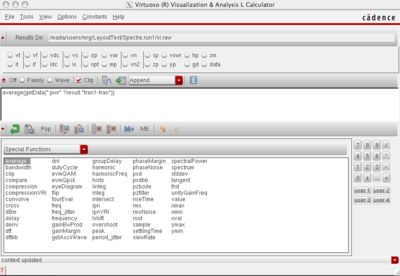
| + | You can then plot the power in the waveform viewer. It will be shown with all the other signals. In order to find the average power, you select :pwr and click on the calculator option instead of the plot option. In the calculator window, select "average" in the special functions. Then select the "Evaluate" button. (It is on the right of the "Clip" option and to the left of the Table and Append options). This will give you the average power in Watts. | ||
| + | |||
| + | [[Image:spectrePower.jpg|400px]] | ||
| + | |||
| + | |||
| + | To enable power analysis in hspice | ||
| + | :1) go to Simulation->Analog Options->All | ||
| + | This will open a dialog box listing various Hspice analysis commands and fields for their values. | ||
| + | Refer to Hspice documentation before using any of these options | ||
| + | |||
| + | == Documentation == | ||
| + | |||
| + | Finally, for more help... | ||
| + | |||
| + | :Open file: /projects/cmpe122/software/synopsys/I-2013.12-1/hspice/docs_help/hspice_sa.pdf | ||
Latest revision as of 22:37, 24 December 2020
There are many ways to simulate from Virtuoso. Which one is best depends on your PDK and your final goals.
Contents
[hide]Setting up analogLib
Before you start virtuoso, make sure to add the analogLib to your libraries. Do this by editing cds.lib in your home directory (or in the project directory). You should see something like this:
DEFINE analogLib $CDSHOME/tools/dfII/etc/cdslib/artist/analogLib
DEFINE US_8ths   $CDSHOME/tools/dfII/etc/cdslib/sheets/US_8ths
DEFINE basic     $CDSHOME/tools/dfII/etc/cdslib/basic
DEFINE cdsDefTechLib $CDSHOME/tools/dfII/etc/cdsDefTechLib
DEFINE NCSU_TechLib_FreePDK45  $PDK_DIR/ncsu_basekit/lib/NCSU_TechLib_FreePDK45
DEFINE NCSU_Devices_FreePDK45  $PDK_DIR/ncsu_basekit/lib/NCSU_Devices_FreePDK45
DEFINE cmpe_222_lib /mada/users/rsankara/cmpe_222_lib
In case your cds.lib does NOT have analogLib or one of the above libraries, then add it as follows:
DEFINE analogLib $CDSHOME/tools/dfII/etc/cdslib/artist/analogLib
Save the file and start virtuoso. You should see a new library in the library manager.
Select Analog Environment
With the schematic file open, hspice can be invoked from within Virtuoso.
- Select Launch → ADE L.
Select Simulator (hspiceD)
Virtuoso Analog Design Environment supports various simulators such as hspiceD, Spectre, and Ultrasim. hspiceD was previously chosen. Now, run
- Select Setup → Simulator/Directory/Host.
A follow up window will pop up giving your simulator options. Select hspiceD. Also specify a run directory. Press ok.
Simulation Run Directory indicates where your simulation files will be stored. The generated netlist file will be stored within in a file called "netlist". All of the other options necessary for running the simulation are stored in this directory as well in the form of separate files like netlistHeader, netlistFooter. When you run the simulation, all the options are put together by the simulator. This is useful for storing separate simulation setups for different parts of your design.
Choosing Analysis Type and Length
From the Analog Environment window
- Select Analysis → Choose
Make sure to select tran and specify an appropriate stop time and time step (example 1ns). The start time is typically 0. Be sure to choose a stop time that is greater than the period of the input signal. Hspice supports the SI prefixes so 500n would be 500 nano seconds.
Adding Model Library Files
The next step is to add the spice data for the simulator.
- Select Setup → Model Library Setup .
We will be adding the data for the NMOS and PMOS transistor.
If you are using FreePDK as your Process Design Kit,
Click on Add File and add these files:
$PDK_DIR/ncsu_basekit/models/hspice/tran_models/models_nom/NMOS_VTL.inc
$PDK_DIR/ncsu_basekit/models/hspice/tran_models/models_nom/PMOS_VTL.inc
Select OK when finished.
These paths will be automatically written as ".include" into a file called input.ckt
If you are using SCMOS(TSMC_02d) as your Process Design Kit,
Click on Add File and add these files instead:
/mada/software/techfiles/ncsu/models/hspice/public/tsmc18dP.m
/mada/software/techfiles/ncsu/models/hspice/public/tsmc18dN.m
Select OK when finished.
Perform this Adding Model Library Files step only for the process you are supposed to use. Adding multiple process files may lead to simulation problems.
Running Simulation
To run a simulation, first select the type of analysis in Analysis → Choose... For a transient, specify the stop time (e.g. 1n).
It is easier to not add voltage sources to the inputs directly and instead make stimulus in a file. You can edit a stimulus file directly and include it in your simulation. Create a text file named stimulus.sp in your simulation directory and create something like this in it:
// Stimulus Statements Hspice format
.global VDD! vdd! GND! gnd!
vdd vdd! 0 vhigh
.param vhigh=1200mV
.param vlow=0
.param tdelay=0n
.param trise=5p * pick a reasonable value
.param tfall=5p * pick a reasonable value
.param tpulse = 10n
v_A  A  0 pat (vhigh vlow tdelay trise tfall tpulse  b01010101  rb=1 r=1)
C_Z Z     0 100fF * pick a reasonable value
The above statements define the global signals, define the vdd voltage using a parametrized statement and also some timing values. These statements may also be written in the netlist file itself if you wish to have it all in a single file. The .param statements above are used for parameterizing simulation variables. This way, if you wish to change some values for simulation, you only need to change it in the .param statement and it will take effect throughout. The v_A is a voltage source statement producing a bit stream of 01010101 as stimulus with rise,fall and pulse width times defined in the .param statements. Save the file you have now created as stimulus.sp and store it in your simulation directory.
To specify the stimulus, select Setup → Simulation Files... and provide the path to your stimulus.sp.
For more information on Hspice commands you can look at the manual:
/projects/cmpe122/software/I-2013.12-1/hspice/docs_help/hspice_sa.pdf
Ouput Window
Before Running, select Output → Save All... to save all schematic data. (Note, this might not be best on big designs!) Or, you can select Outputs → To Plot → Select on Schematic and then click on all of the items on the schematic.
Then,
- Select Simulation → Run
This will generate the netlist file, run the simulation, and save the results for the waveform viewer. You should re-run this every time you change your schematic.
You can also select Simulation → Create Raw to create the raw simulation file for debugging. You should be able to see your include stimulus, netlist, and a bunch of other stuff.
If this pops up a window that says it failed, fix the previous options. You need to debug this by looking at the output of the simulator in si.log (which is the output of running the simulator, if the simulator failed to run) or si.out (which is the actual simulator output if it ran successfully, but simulation may have failed). This will show you if it even got to the point of running the simulator.
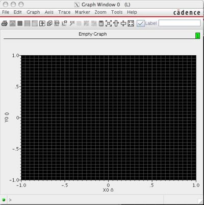
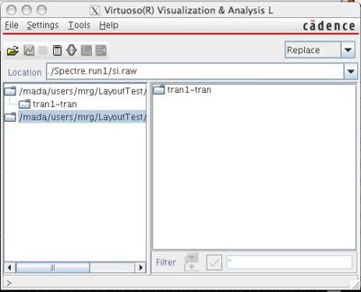
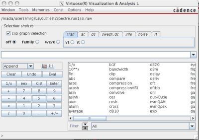
If it succeeded, you can select Tools → Waveform . When you do this, you get three windows:
Select the "File Open" icon and then find the appropriate "raw" result file in the browser. This should open the data in the browser. Double click on the transient simulation directory and you should see signal names that correspond to your design. Double click on "A" to add it. Change the upper right option to "Append" and double click on "Z" to add it as well. If you don't change the option, it will replace the A waveform with Z. If there are problems with vdd! and gnd! you can debug that here.
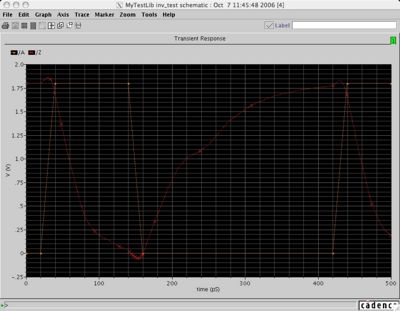
You should get something that looks similar to this in the graph window:
Note that your signals should always rise to full vdd (1.2V) and down to gnd (0V) or else something is wrong with your logic. This is CMOS so everything is "rail to rail". It is likely an unconnected supply voltage or floating body.
Waveform - Zooming and Trace
With the waveform window open, you can zoom in and find exact values.
Zoom
- Select Zoom → X Zoom .
- Now click and drag in the waveform window to select the x-range you want to zoom to.
Tracing
- Select Marker → Place → Trace Marker
- Click on one of the waveforms in the window. This places a small label on the waveform. You can drag this marker anywhere on the waveform.
Separate Windows
- Sometimes the window will get too cluttered. You can plot each signal in a separate window by clicking the 4th icon in the toolbar from the left to put it in "Strip Mode".
Reloading
- If you make a change and resimulation, you can simply click File → Reload
Exporting Tip
- If you intend to export the plot, it would be wise to change the background color to something other than black. In addition you can change the width of the lines by right clicking on the line and selecting properties.
Power/Energy Analysis
To enable power analysis in hspice, add this statement to your stimulus file:
.measure tran toplvl_avg_power avg   power from=0ns to=100ns
.measure tran toplvl_avg_energ integ power from=0ns to=100ns
.measure tran toplvl_avg_current avg I(VDD) from=0ns to=100ns
For more information on the .measure syntax, please refer hspice user guide at:
/projects/cmpe122/software/synopsys/I-2013.12-1/hspice/docs_help/hspice_sa.pdf
You can then plot the power in the waveform viewer. It will be shown with all the other signals. In order to find the average power, you select :pwr and click on the calculator option instead of the plot option. In the calculator window, select "average" in the special functions. Then select the "Evaluate" button. (It is on the right of the "Clip" option and to the left of the Table and Append options). This will give you the average power in Watts.
To enable power analysis in hspice
- 1) go to Simulation->Analog Options->All
This will open a dialog box listing various Hspice analysis commands and fields for their values. Refer to Hspice documentation before using any of these options
Documentation
Finally, for more help...
- Open file: /projects/cmpe122/software/synopsys/I-2013.12-1/hspice/docs_help/hspice_sa.pdf
